Usage#
This page aims to provide a brief overview of JAQSI (just another quantum simulator).
Circuits are built by calling gates inside a plain Python function and are executed through the Script class.
Frameworks layered on top of JAQSI (such as qml-essentials, which builds quantum Fourier models on it) usually abstract the simulator away entirely, but building custom circuits with more granular control is a first-class use case.
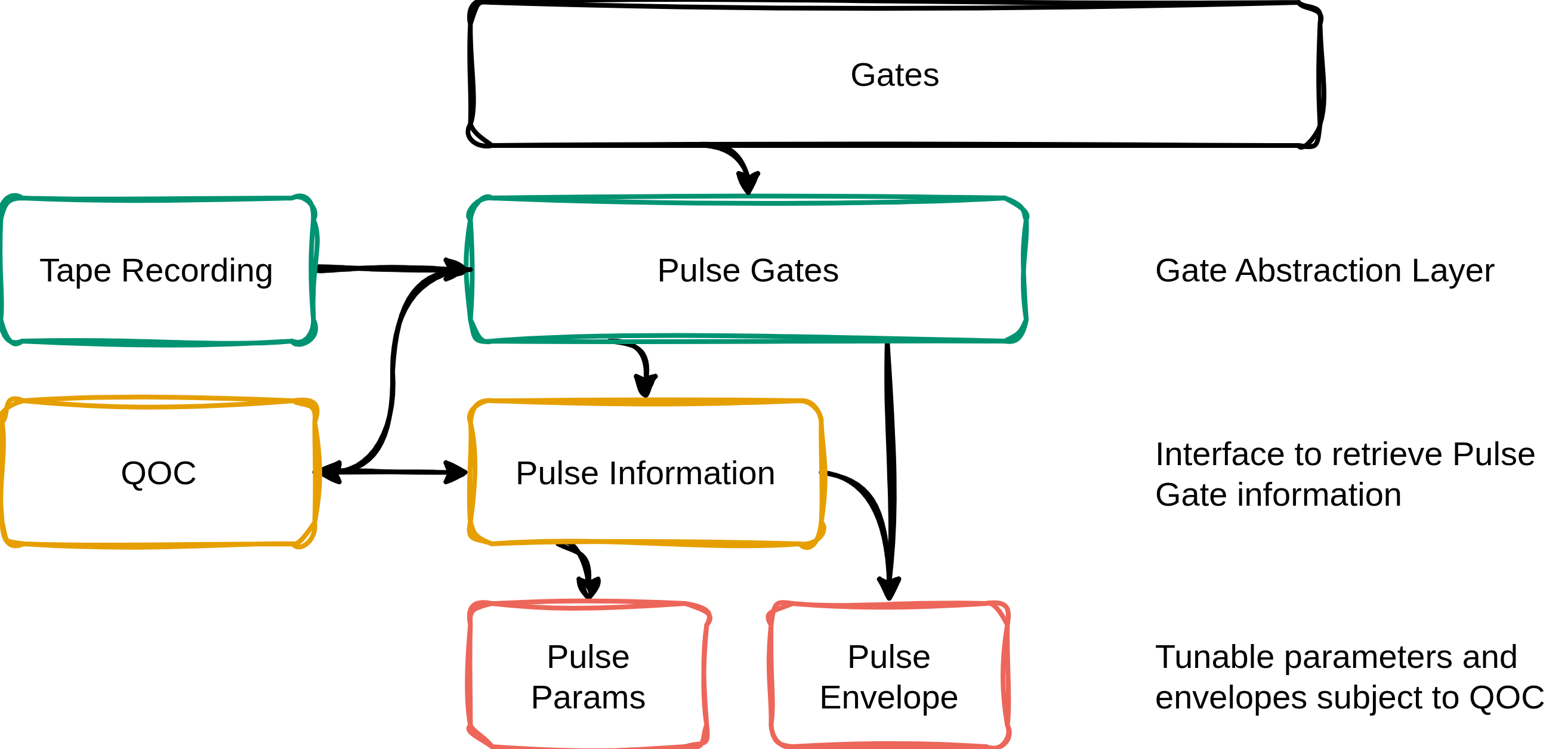
In the figure below, you can see how JAQSI provides the foundation for the more standard interfaces Model, Ansaetze and Gates.
The circuit-constructing layers interface with the Operations module of JAQSI, while Model interfaces with the Script class, the main interface for circuit execution.
Generally, all operations are registered on a Tape when being created in the context of a Script (see examples below).
All gate matrix definitions are registered in the Gateset module, the Kraus channels for noisy simulation in Noise, and the shared Operation machinery in Operations.


While the standard gate execution is quite straightforward, the pulse simulation requires a bit more care.
Here we split up PulseGates (abstracted by the Gates class) into PulseParams and PulseEnvelope to get more fine-grained control over the underlying implementation.
As a single source of truth for both, there is the PulseInformation class, providing valid combinations of these two characteristics.
Architecture#
Internally, the simulator is split into a handful of modules, each with a single responsibility. Together they form a pipeline that turns a circuit function into a measurement result.
operations.py: the foundation. Defines theOperationbase class that every gate, observable and noise channel derives from, together with the (parametrized) Hamiltonians used for pulse evolution. EachOperationcarries its matrix definition and knows how to apply itself to a statevector or density matrix via cachedeinsumcontractions.gates.py: the entry point for applying gates.Gates.<Name>(...)records a gate on the tape, attaches any requested noise, and routes the call toUnitaryGatesorPulseGatesdepending on thepulseflag. Write circuits against this and they run at either level unchanged.unitary.py: the ideal-unitary backend. Builds thegatesetoperation for each gate and attaches the requested noise channels; also home to theGateErrorangle noise and thebatch_gate_errorflag.pulses.py: the pulse-level backend. Implements the fundamental gates (RX, RY, RZ, CZ) as time-dependent drives and composes the rest from them, withPulseParams,PulseEnvelopeand the globalPulseInformationcalibration state.gateset.py: the gate library. Every concrete gate (H,RX,CX,Rot,PauliRot, ...) and observable (PauliZ, ...) as anOperationsubclass, so instantiating one inside a circuit function records it on the active tape.paulis.py: the symbolic Pauli/Clifford layer. A stabilizer-tableauPauliWordwith O(n) Clifford conjugation plus the matrix-based decomposition helpers it replaces. Symbolic bookkeeping in integer NumPy rather than numeric simulation; it backs Pauli-Clifford circuit transforms and Fourier-tree algorithms built on top of JAQSI.noise.py: the Kraus noise channels (BitFlip,DepolarizingChannel,AmplitudeDamping,ThermalRelaxationError, ...), layered onOperation. Recording any of them on a tape is what switches the simulation from statevector to density matrix.tape.py: the recording layer. Holds the thread-localTapeonto which operations register themselves as they are created. Arecording()context manager collects the operations built inside a circuit function into an ordered list; nothing is executed yet.script.py: the orchestrator. TheScriptclass is the entry point for executing a circuit (and whatModelbuilds upon), the counterpart toGatesfor building one. It records the circuit, infers the number of qubits, decides between pure and density-matrix simulation, dispatches measurements, and takes care of JIT caching, automatic batching (vmapwith memory-aware chunking) and circuit drawing.simulation.py: the compute engine. A set of pure, stateless functions that run a recorded tape:simulate_pure(statevector),simulate_mixed(density matrix) and the measurement kernels (measure_state,measure_density,sample_shots). Before simulating,simulate_and_measureresolves the pulse-level gates of the tape throughevolution.resolve_pending. Being pure JAX functions, they are fully differentiable andjit/vmap-compatible.memory.py: memory accounting. Pure helpers that estimate the peak memory of a batched run and, when it would not fit in available RAM, split the batch into chunks that do (estimate_peak_bytes,compute_chunk_size,execute_chunked).Scriptcalls these to drive its memory-awarevmapchunking.drawing.py: rendering. Turns a recorded tape into a text, matplotlib or TikZ circuit diagram, and pulse events into a pulse-schedule plot.evolution.py: Hamiltonian time-evolution. TheEvolutionclass builds gates that evolve a (parametrized) Hamiltonian in time, either analytically (exp(-i t H)for a staticH) or by solving the Schrödinger equation with an adaptivediffraxsolver or a fixed-step Magnus integrator. Time-dependent gates are returned as lazyPendingEvolutionoperations;resolve_pendingsolves all pending gates of a tape in one batched call per pulse shape, optionally on the host CPU (host_offload). This module backs the pulse-level simulation.__init__.py: the package entry point. Re-exportsScriptfor circuit building,Gatesfor applying them, theHamiltonianfactory for time-evolution sources, and the quantum-info helpers, so thatimport jaqsiis enough for everyday use. Time evolution is invoked as a method on the Hamiltonian object (hamiltonian.evolve(...)); theEvolutionengine is re-exported for solver configuration (Evolution.set_solver_defaults).math.py: model-agnostic quantum-info utilities on states and density matrices:fidelity,trace_distance,phase_difference,logm_v, the quantum Fisher information and Fubini-Study metric, plus the pulse/gate-independent post-processing helperspartial_traceandmarginalize_probs.qoc.py: quantum optimal control. Optimizes pulse parameters against a target unitary with a configurable cost-function registry, and ships the tuned results asqoc_results_<envelope>.csvpackage data.
A call to Script.execute(...) then runs four stages:
- Record : the circuit function is executed once so that each operation registers itself on a fresh
Tape. - Prepare : the qubit count is inferred and the presence of noise channels decides between statevector and density-matrix simulation.
- Simulate : the operations are applied in order, each gate contracted into the state via
einsum. - Measure : the resulting state is turned into the requested output (
state,probs,expvalordensity) and optionally sampled into shots.
As the whole pipeline is built on JAX, any execution can be differentiated, JIT-compiled and vectorized.
Usage#
The API of our simulator is very similar to what one might be used to from PennyLane.
Gate Level#
Gates is the entry point for applying gates.
Calling Gates.<Name>(...) inside a circuit function records the gate on the active tape,
attaches any requested noise, and routes the call to the unitary or the pulse backend.
Write circuits against Gates and the same circuit runs at either level; see
pulse level below.
For a basic circuit execution, we have to do two imports:
Next, we can create a circuit and specify the observable:
def circuit():
    Gates.H(wires=0)
    Gates.CX(wires=[0, 1])

obs = [js.PauliZ(wires=0), js.PauliZ(wires=1)]
Observables are the one place you reach past Gates: an observable is an object you hand to
execute, not a gate you apply, so it comes straight from the package root (equivalently
jaqsi.gateset).
Finally, creating a Script and executing it will give us the probabilities for this standard Bell circuit:
Parameterization of circuits is straightforward; you just have to pass the args to the execute function:
import jax.numpy as jnp

n_qubits = 1

def circuit(phi, theta, omega):
    Gates.Rot(phi, theta, omega, wires=0)
    Gates.Rot(jnp.pi, 1/2*jnp.pi, 1/4*jnp.pi, wires=0)

obs = [js.PauliZ(wires=i) for i in range(n_qubits)]
jss = js.Script(circuit)
jss.execute(type="expval", obs=obs, args=(jnp.pi, 1/2*jnp.pi, 1/4*jnp.pi))
Training those circuits is a breeze as we entirely build upon JAX and can just use Optax for this purpose:
import jax
import optax as otx

def cost_fct(params):
    phi, theta, omega = params
    return jss.execute(type="expval", obs=[js.PauliZ(0)], args=(phi, theta, omega))[0]

params = jax.numpy.array([0.1, 0.2, 0.3])
opt = otx.adam(0.01)
opt_state = opt.init(params)

for epoch in range(1, 101):
    grads = jax.grad(cost_fct)(params)
    updates, opt_state = opt.update(grads, opt_state, params)
    params = otx.apply_updates(params, updates)

    if epoch % 10 == 0:
        print(f"Epoch: {epoch}, Cost: {cost_fct(params):.4f}")
See the training page for the JIT-compiled version of this loop, fitting data with batched inputs, and optimizing pulse parameters.
Gates.<Name>(...) records the gate and returns nothing. When you need the operation
object itself — to call .dagger() or .power() on it, to build a composite observable,
or to do matrix algebra — take the class from jaqsi.gateset instead:
from jaqsi.gateset import RX, PauliX

def circuit():
    RX(0.5, wires=0)
    RX(0.5, wires=0).dagger()
    PauliX(wires=0).power(2)

obs = [js.PauliZ(0)]
jss = js.Script(circuit)
res = jss.execute(type="expval", obs=obs)

print(res) # we expect to end up in |0⟩ again
Noise is normally requested per gate through Gates, which emits the matching channels
for you (see noise):
noise_params = {"Depolarizing": 0.1}

def circuit():
    Gates.H(wires=0, noise_params=noise_params)
    Gates.CX(wires=[0, 1], noise_params=noise_params)

jss = js.Script(circuit)
rho = jss.execute(type="density")
purity = jnp.real(jnp.trace(rho @ rho))
print(purity) # Purity should be < 1
Channels are operations too, so they can also be placed by hand from jaqsi.noise when you
want control over exactly where they land.
By default the simulation starts from the all-zero state \(\lvert 0\dots0\rangle\).
To start from an arbitrary statevector instead, pass it via the initial_state
argument of execute:
def circuit():
    Gates.RX(0.3, wires=0)

jss = js.Script(circuit)
plus = jnp.array([1.0, 1.0], dtype=complex) / jnp.sqrt(2.0)  # |+⟩
res = jss.execute(type="expval", obs=[js.PauliZ(0)], initial_state=plus)
Without in_axes the state must be a single statevector of shape (2**n,).
When batching with in_axes, initial_state may be a single 1D state broadcast across the batch, or a 2D array of shape (B, 2**n) that provides one state per sample.
Pulse Level#
This section focuses on the pulse-level interface of the simulator. For pulse gate mechanics, envelopes and quantum optimal control, head over to the pulses documentation.
Pulse-level simulation goes through the same entry point: pass pulse=True to any gate and
Gates routes it to the pulse backend instead of the ideal unitary.
Nothing else about the circuit changes.
def circuit(w):
    Gates.RX(w, wires=0, pulse=True)

obs = [js.PauliZ(0)]
jss = js.Script(circuit)
res = jss.execute(type="expval", obs=obs, args=(jnp.pi*0.5,))
print(res) # expect sth. around 0 (but not too close)
Because the flag is per call, a circuit can mix both levels — here the entangling gate stays ideal while the rotations are lowered to pulses:
def circuit(w):
    Gates.RX(w, wires=0, pulse=True)
    Gates.RY(w, wires=0, pulse=True)
    Gates.CX(wires=[0, 1])
Mixing pulse-level simulation with noisy simulations is possible as well:
noise_params = {"Depolarizing": 0.1}

def circuit(w):
    Gates.RX(w, wires=0, pulse=True, noise_params=noise_params)
    Gates.RY(w, wires=0, pulse=True, noise_params=noise_params)
    Gates.CX(wires=[0, 1], noise_params=noise_params)

jss = js.Script(circuit)
rho = jss.execute(type="density", args=(jnp.pi*0.5,))
purity = jnp.real(jnp.trace(rho @ rho))
print(purity) # Purity should be < 1
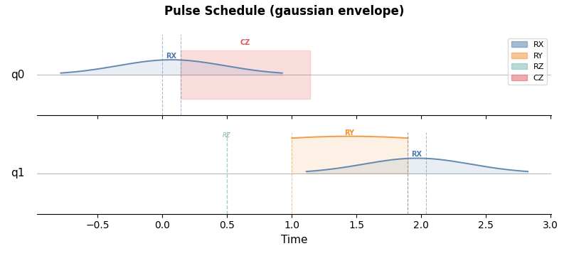
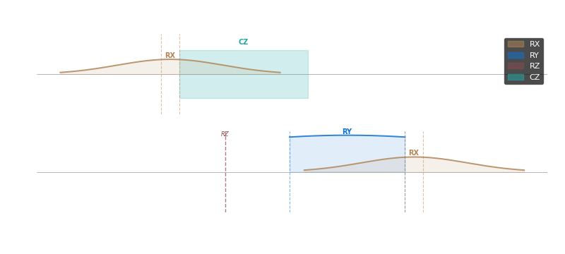
You can visualize the pulse schedules, i.e. the sequence in which the pulses are applied on each qubit in the circuit, using the draw method.
Here, shaded areas represent the pulse shape/envelope (e.g. "Gaussian") of the pulse and the vertical line represents the time at which the pulse is applied.
Note that all gates are automatically decomposed into basis gates (e.g. H is decomposed into RZ and RY).
def circuit(w):
    Gates.RX(w, wires=0, pulse=True)
    Gates.CZ(wires=[0, 1], pulse=True)
    Gates.H(wires=1, pulse=True)
    Gates.H(wires=1, pulse=True)

jss = js.Script(circuit)

fig, axes = jss.draw(figure="pulse", args=(jnp.pi*0.5,))
Now let's get a level deeper into the pulse interface. Under the hood, running a pulse gate means evolving a Hermitian matrix in time. To demonstrate this, we build a very simple circuit:
def evol_circuit(t):
    time_evol = js.Hermitian(matrix=js.PauliZ._matrix, wires=0).evolve()
    time_evol(t=t, wires=0)
We can use this circuit directly in JAQSI by passing it to the Script class we've seen above:
Here, we let the circuit evolve for t=0.3 and measure the qubit in the X basis.
Obviously this isn't particularly useful, because it doesn't change the state of the qubit.
However, we can extend this circuit a little bit to start in the |+⟩ state instead:
def evol_circuit(t):
    Gates.H(wires=0)  # prepare |+⟩
    time_evol = js.Hermitian(matrix=js.PauliZ._matrix, wires=0).evolve()
    time_evol(t=t, wires=0)
Note how we combine a "standard" gate with a Hermitian evolution. We can then measure:
t = 0.3
jss = js.Script(f=evol_circuit)
res = jss.execute(type="expval", obs=[js.PauliX(0)], args=(t,))
which gives us exactly jnp.cos(2 * t).
We've just seen an example for a static Hermitian evolution. Naturally we can extend this to a parameterized Hermitian as well:
def coeff(p, t):
    return p

def circuit(p, t):
    Gates.H(wires=0)  # prepare |+⟩
    ph = coeff * js.Hermitian(matrix=js.PauliZ._matrix, wires=0, record=False)
    ph.evolve()([p], t)
Note here that coeff is a callable.
While it seems a little bit strange to first use a callable and then parameterize it directly afterwards, this mechanism allows us to pre-compile the operation.
p = 0.5
jss = js.Script(f=circuit)
res = jss.execute(type="expval", obs=[js.PauliX(0)], args=(p, t))
Naturally, we can now use this parameter in a training scenario and leverage the performance advantage we got through the pre-compilation.