Pulses#
Our framework allows constructing circuits at the pulse level, where each gate is implemented as a time-dependent control pulse rather than an abstract unitary.
This provides a more fine-grained access to the simulation of the underlying physical process.
While we provide a developer-oriented overview in this section, we would like to highlight Tilmann's Bachelor's Thesis if you want to have a more detailed read into pulse-level simulation and quantum Fourier models.
Note that we support GPU-accelerated pulse-level simulation, but keep in mind that pulse-level ODE solves are latency-bound on a GPU.
This means that jaqsi.Evolution.set_solver_defaults(host_offload=True) keeps them on the CPU while the circuit runs on the GPU, which pays off below roughly a thousand solves per call (forward simulation and eager gradients; not inside a jitted gradient).
The following three points can help you make a decision on when to run what on which device with or without the host_offload flag:
- Small batch, low num. qubits: CPU-only is fastest. The flag makes the GPU the second-best option instead of the worst, but it cannot beat the CPU because the gate part is trivial and the offload adds a round trip.
- Small batch, large num. qubits: Gate part starts to dominate and favors the GPU (16 qubits: 5.1 ms on CPU vs 0.6 ms on GPU at gate level). Here the flag should beat CPU-only.
- Large batch (above roughly a thousand solves per call): GPU with the flag off is fastest, and with the flag on, CPU speed is expected.
We implement a fundamental set of gates (RX, RY, RZ, CZ) upon which other, more complex gates can be built.
The dependency graph is shown in the following figure:
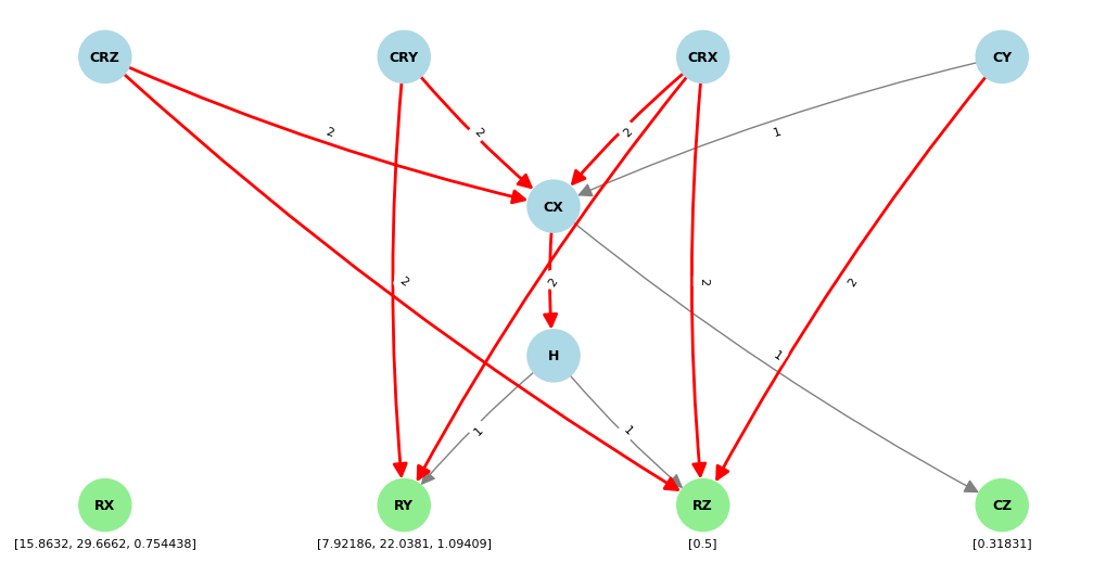
 In this graph, the edge weights represent the number of child gates required to implement a particular gate.
The gates at the bottom represent the fundamental gates.
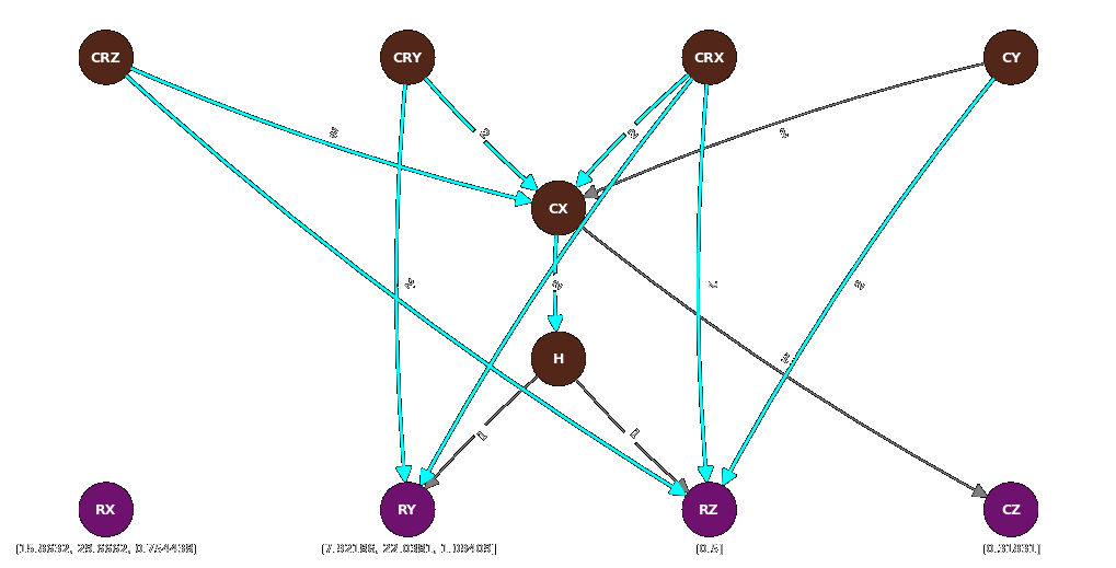
In this graph, the edge weights represent the number of child gates required to implement a particular gate.
The gates at the bottom represent the fundamental gates.
Pulse gates are reached through the same entry point as every other gate, Gates.
Pulse simulation is enabled per call by adding the pulse=True keyword argument, e.g.:
Because the flag lives on the call, the same circuit function can run at either level, and a
circuit can mix the two. Calling PulseGates directly bypasses the noise handling and
pulse-parameter management that Gates performs, so prefer the flag.
Pulse Parameters per Gate#
You can use the PulseInformation class in jaqsi.gates to access both the number and optimized values of the pulse parameters for each gate.
Consider the following code snippet:
from jaqsi.gates import PulseInformation as pinfo

gate = "CX"

print(f"Number of pulse parameters for {gate}: {pinfo.num_params(gate)}")
# Number of pulse parameters for CX: 11

gate_instance = pinfo.gate_by_name(gate)

print(f"Childs of {gate}: {gate_instance.childs}")
# Childs of CX: [H, CZ, H]

print(f"All parameters of {gate}: {len(gate_instance.params)}")
# All parameters of CX: 11

print(f"Leaf parameters of {gate}: {len(gate_instance.leaf_params)}")
# Leaf parameters of CX: 6
Looking back at the dependency graph, we can easily see where the discrepancy between the overall number of parameters and the number of leaf parameters comes from. The CX gate is composed of two Hadamard gates, which in turn are decomposed into RY and RZ gates. By default, our implementation assumes that you want to treat each rotational gate equally, thus the number of leaf parameters is just the "unique" number of parameters resulting after merging multiple occurrences of the same gate type. However, it is also possible to override this behavior, as we will see in the following example.
Calling Gates in Pulse Mode#
To execute a gate in pulse mode, provide pulse=True when calling it on Gates.
Optional pulse_params can be passed; if omitted, optimized default values are used:
w = 3.14159

# CX gate with default optimized pulse parameters
# (gates of equal type will receive equal pulse parameters)
Gates.CX(wires=[0, 1], pulse=True)

# CX gate with custom pulse parameters (overwriting default pulse parameters)
pulse_params = pinfo.gate_by_name("CX").params * 1.1
Gates.CX(wires=[0, 1], pulse=True, pulse_params=pulse_params)

# RX gate with a rotation angle and default pulse parameters
Gates.RX(w, wires=0, pulse=True)
Pulse Envelopes and Solver#
Each pulse is shaped by an envelope. The available envelopes can be queried with PulseEnvelope.available():
from jaqsi.gates import PulseEnvelope

print(PulseEnvelope.available())
# ['gaussian', 'square', 'cosine', 'drag', 'sech', 'general']
The default is drag. The envelope is a process-global setting, switched with PulseInformation.set_envelope("gaussian").
Parameter counts depend on the envelope; the counts above are for drag.
Under the hood, pulse gates are simulated by integrating their time-dependent Hamiltonian. The ODE solver can be configured via Evolution.set_solver_defaults, where solver is one of "dopri8" (default), "dopri5", "magnus2" or "magnus4":
The magnus_steps argument sets the number of fixed substeps for the Magnus integrators and is ignored for the adaptive Dormand-Prince solvers (dopri8, dopri5).
Note that pulse gates are solved lazily when the circuit is simulated. This means that all gates of a tape that share a pulse shape are integrated in one batched solve, and gates with identical parameters (the same fixed-angle rotation on several wires, every CZ) are solved only once. This keeps compile times short and matters most on a GPU, where each separate solve costs a few milliseconds of launch latency.
Quantum Optimal Control#
Our package provides a Quantum Optimal Control (QOC) interface for directly optimizing pulse parameters for specific gates.
Conceptually the provided QOC class contains methods to create test circuits (create_GATE) which return two circuits, one using the pulse-level implementation of GATE and the other using the unitary-level implementation of GATE.
For the specific implementation of these methods, we refer to the documentation of the QOC class.
To test a broad range of states, each of these circuits includes not only GATE itself but also other, unitary-based gates.
Those usually take a parameter w, allowing one to sweep through the parameter space and validate whether GATE actually mimics its unitary counterpart.
Using the standard parameter specification, we can initialize the QOC class:
For a detailed description of available arguments, we refer to the documentation of the QOC class.
Now, we can select gates by passing sel_gates=["GATE"] when calling optimize_all:
which will run the optimization for the specified gates.
The output of the optimization is logged to qoc_logs.csv whereas the resulting pulse parameters are stored in qoc_results_<envelope>.csv.
Internally, a multi-objective cost function is utilized to tune the pulse parameters of the basis gates.
Primarily, the fidelity between the pulse gate and a target unitary is optimized, but the default setting also takes into account the width of the pulse and a time normalization.
For the exact weighting between these cost functions, we refer to default_qoc_params.
Besides the cost functions and their respective weights, you can also specify the envelope used for the pulse gate.
For further examples we refer to our "Pulses" notebook.
With the optimized pulse parameters we can generate a fidelity plot as follows:
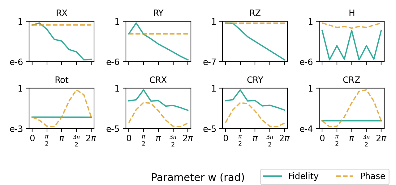
Note that in this plot, the phase error is shown as \(1-\text{phase error}\) to align it with the fidelity scale.