Training#

This section describes how to use the model provided with this package, using a simple training scenario as an example.

We consider a Fourier series with \(n\) frequencies defined as follows:

Here, \(\omega \in \boldsymbol{\Omega}\) are the frequencies in the spectrum with the Fourier coefficients \(c_{\omega}(\boldsymbol{\theta})\), parameterized by the set of trainable parameters \(\boldsymbol{\theta}\).

As shown by Schuld et al. (2020), a quantum circuit, parametrised by \(\boldsymbol{\theta}\) and input \(x\) and is equivalent to the Fourier series representation. Such circuits must be of the following form:

Therefore, training such a model on a Fourier series is a proof-of-concept which we want to demonstrate here.

Let's start with building our dataset. A Fourier series with \(4\) frequencies:

import pennylane.numpy as np
import matplotlib.pyplot as plt

domain = [-np.pi, np.pi]
omegas = np.array([1, 2, 3, 4])
coefficients = np.array([0.5, 0.5, 0.5, 0.5])

# Calculate the number of required samples to satisfy the Nyquist criterium
n_d = int(np.ceil(2 * np.max(np.abs(domain)) * np.max(omegas)))
# Sample the domain linearly
x = np.linspace(domain[0], domain[1], num=n_d)

# define our Fourier series f(x)
def f(x):
    return 1 / np.linalg.norm(omegas) * np.sum(coefficients * np.cos(omegas.T * x))

# evaluate f(x) on the domain samples
y = np.stack([f(sample) for sample in x])

plt.plot(x, y)
plt.xlabel("x")
plt.ylabel("f(x)")
plt.show()

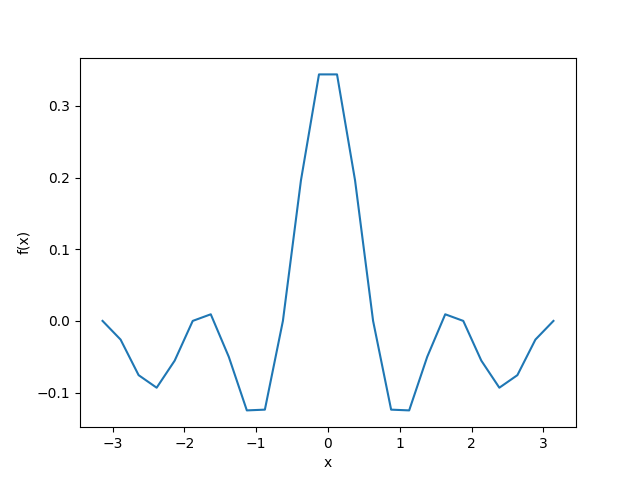
Note that we chose the coefficients to be all \(0.5\). Play around with those values to change the magnitude of each frequency component. Also note that we're using the Pennylane version of Numpy, which is required because of the optimizer that we will be using later. Now that we have our "dataset", let's move on and build a model:

from qml_essentials.model import Model

model = Model(
    n_qubits=4,
    n_layers=1,
    circuit_type="Circuit_19",
)

This is the minimal amout of information needed. According to the work referenced above, a model with \(4\) qubits should be capable of learning a Fourier series with \(4\) frequencies, considering single qubit Pauli encoding (which we have by default).

Now, let's train our model:

import pennylane as qml

opt = qml.AdamOptimizer(stepsize=0.01)

def cost_fct(params):
    y_hat = model(params=params, inputs=x, force_mean=True)

    return np.mean((y_hat - y) ** 2)

for epoch in range(1, 1001):
    model.params, cost_val = opt.step_and_cost(cost_fct, model.params)

    if epoch % 100 == 0:
        print(f"Epoch: {epoch}, Cost: {cost_val:.4f}")

plt.plot(x, y, label="True function")
plt.plot(x, model(params=model.params, inputs=x, force_mean=True), label="Model prediction")
plt.xlabel("x")
plt.ylabel("f(x)")
plt.legend()
plt.show()

To compile the whole training step with jax.jit, build the cost function on model.apply instead of calling the model directly (see Usage).

Epoch: 100, Cost: 0.0081
Epoch: 200, Cost: 0.0073
Epoch: 300, Cost: 0.0051
Epoch: 400, Cost: 0.0043
Epoch: 500, Cost: 0.0036
Epoch: 600, Cost: 0.0022
Epoch: 700, Cost: 0.0014
Epoch: 800, Cost: 0.0008
Epoch: 900, Cost: 0.0006
Epoch: 1000, Cost: 0.0001

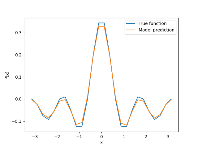
As you can see, the model is able to learn the Fourier series with the \(4\) frequencies.

Trainable frequencies#

For the model we just trained, we considered the best possible scenario: evenly spaced, integer omegas. But, as shown by Schuld et al. (2020), we'll need an increasing and inefficient amount of qubits for larger omegas. What is more, the model will fail altogether if the frequencies are un-evenly spaced. Luckily, Jaderberg et al. (2024) showed how we can let the model choose its own frequencies by including a set of encoding parameters that act on the input before the encoding layers of the circuit. We demonstrate this functionality below.

First, let's slighly modify the omegas from the first example and re-generate the data:

domain = [-np.pi, np.pi]
omegas = np.array([1.2, 2.6, 3.4, 4.9])
coefficients = np.array([0.5, 0.5, 0.5, 0.5])

# Calculate the number of required samples to satisfy the Nyquist criterium
n_d = int(np.ceil(2 * np.max(np.abs(domain)) * np.max(omegas)))
# Sample the domain linearly
x = np.linspace(domain[0], domain[1], num=n_d)

# define our Fourier series f(x)
def f(x):
    return 1 / np.linalg.norm(omegas) * np.sum(coefficients * np.cos(omegas.T * x))

# evaluate f(x) on the domain samples
y = np.stack([f(sample) for sample in x])

plt.plot(x, y)
plt.xlabel("x")
plt.ylabel("f(x)")
plt.show()

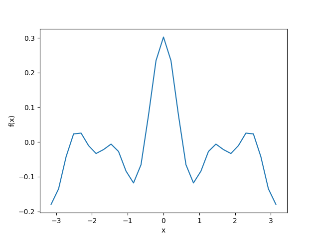
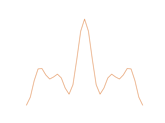
Now, let's build a model with fixed frequencies, as before, and one with trainable frequencies:

model = Model(
    n_qubits=4,
    n_layers=1,
    circuit_type="Circuit_19",
)
model_tf = Model(
    n_qubits=4,
    n_layers=1,
    circuit_type="Circuit_19",
    trainable_frequencies=True # <---!
)

Let's train both models:

# - Fixed Frequencies -
opt = qml.AdamOptimizer(stepsize=0.01)

print("Training fixed frequency model")
for epoch in range(1, 1001):
    model.params, cost_val = opt.step_and_cost(cost_fct, model.params)

    if epoch % 100 == 0:
        print(f"Epoch: {epoch}, Cost: {cost_val:.4f}")

# - Trainable Frequencies -
opt = qml.AdamOptimizer(stepsize=0.01)

def cost_fct_tf(params, enc_params):
    y_hat = model_tf(params=params, enc_params=enc_params, inputs=x, force_mean=True)
    return np.mean((y_hat - y) ** 2)

print(f"\nTraining trainable frequency model")
for epoch in range(1, 1001):
    (model_tf.params, model_tf.enc_params), cost_val_tf = opt.step_and_cost(cost_fct_tf, model_tf.params, model_tf.enc_params)

    if epoch % 100 == 0:
        print(f"Epoch: {epoch}, Cost: {cost_val_tf:.6f}")

plt.plot(x, y, label="True function")
plt.plot(x, model(params=model.params, inputs=x, force_mean=True), label="Fixed frequencies model prediction")
plt.plot(x, model_tf(params=model_tf.params, enc_params=model_tf.enc_params, inputs=x, force_mean=True), label="Trainable frequencies model prediction")
plt.xlabel("x")
plt.ylabel("f(x)")
plt.legend()
plt.show()

Training fixed frequency model
Epoch: 100, Cost: 0.0082
Epoch: 200, Cost: 0.0067
Epoch: 300, Cost: 0.0038
Epoch: 400, Cost: 0.0031
Epoch: 500, Cost: 0.0027
Epoch: 600, Cost: 0.0026
Epoch: 700, Cost: 0.0025
Epoch: 800, Cost: 0.0024
Epoch: 900, Cost: 0.0023
Epoch: 1000, Cost: 0.0023

Training trainable frequency model
Epoch: 100, Cost: 0.008454
Epoch: 200, Cost: 0.002759
Epoch: 300, Cost: 0.002382
Epoch: 400, Cost: 0.001655
Epoch: 500, Cost: 0.000232
Epoch: 600, Cost: 0.000019
Epoch: 700, Cost: 0.000010
Epoch: 800, Cost: 0.000003
Epoch: 900, Cost: 0.000001
Epoch: 1000, Cost: 0.000001

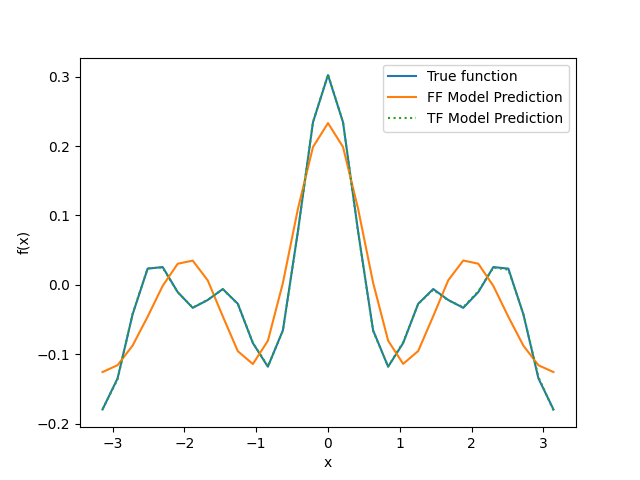
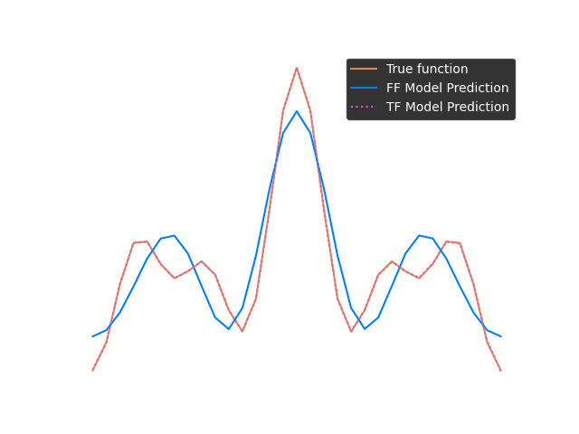
As you can see, the fixed frequencies model was not able to find the underlying function representing the data, while the trainable frequencies model was successful in its training.

Let's quickly check the final encoding parameter of both models:

print(f"Encoding parameters of the fixed frequencies model: {model.enc_params}")
print(f"Encoding parameters of the trainable frequencies model: {np.round(model_tf.enc_params, 3)}")

Encoding parameters of the fixed frequencies model: [1. 1. 1. 1.]
Encoding parameters of the trainable frequencies model: [1.001 2.065 2.817 0.364]

Clearly, the trainable frequencies model found the set of encoding parameters that allowed it to represent the given arbitrary frequency spectrum.

One last thing that might be interesting! Currently, the model applies

enc_params[qubit] * inputs[:, idx]

model.transform_input = lambda inputs, qubit, idx, enc_params: np.arccos(inputs[:, idx])

Using the built-in Dataset#

Previous examples considered a very simplified version of a training dataset. Extending this to multi-dimensional inputs and different encoding schemes of the model can be quite a tedious work to implement. For this purpose, we provide a ready-to-use Fourier series dataset via the Datasets class in the qml_essentials.coefficients module. This dataset uses the model properties to generate a Fourier series that matches what the model can learn, meaning that the frequencies are inferred from model.frequencies. Furthermore, it is possible to control the magnitude of the coefficients, sampled from a complex unit circle, by setting coefficients_min and coefficients_max, and to drop the constant offset by setting zero_centered=True. Calling generate_fourier_series will return the domain samples, Fourier series samples and the coefficients of the Fourier series.

The code snippet below provides a minimal example on how to use this dataset:

import jax
from qml_essentials.coefficients import Datasets

# generate a Fourier series dataset
domain_samples, fourier_samples, coefficients = (
                    Datasets.generate_fourier_series(
                        random_key=jax.random.key(1000),
                        model=model,
                    )
                )

# cost function uses the domain samples as input and compares with the
# Fourier series samples obtained from the dataset
def cost_fct(params):
    y_hat = model(params=params, inputs=domain_samples, force_mean=True)

    return np.mean((y_hat - fourier_samples) ** 2)

for epoch in range(1, 1000):
    model.params, cost_val = opt.step_and_cost(cost_fct, model.params)

    if epoch % 100 == 0:
        print(f"Epoch: {epoch}, Cost: {cost_val:.4f}")

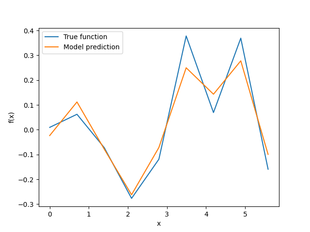
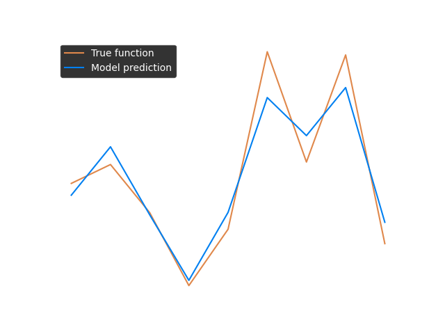
Note that it's more difficult for the model to fit this specific dataset as it, opposed to the previous datasets, also contains complex parts in the coefficients, effectively causing a phase shift.

Off-grid Datasets#

generate_fourier_series composes four building blocks, which you can also call individually if you need more control than the wrapper offers: construct_domain_samples, construct_frequencies, construct_coefficients and calculate_values.

Two of them take arguments that let you build a dataset the model can not represent exactly, which is useful for studying how much a model gains from being able to move its own frequencies.

construct_frequencies accepts an offgrid_mode that displaces components off the model comb, with offgrid_prob setting the likelihood that any single component moves and offgrid_resolution the denominator \(r\) of the offset grid, i.e. offsets are drawn from \(\{\pm j/r\}\) with \(j = 1 \dots r-1\). Mode index displaces each component independently, which spans arbitrary combs that are in general not reachable by the model at all. Mode generator instead displaces the per-gate generator frequencies and rebuilds the comb as their Minkowski sum, which stays reachable by an encoding pulse configuration. Both keep the number of components, the antisymmetry of the comb and the model's frequency range intact. Note that offgrid_prob equals the fraction of off-grid components only in index mode, since a sum of displaced generators can land back on an integer.

construct_domain_samples accepts mts and mfs, following the same convention as Coefficients._fourier_transform, where mts sets how many periods the domain covers and mfs the sample density per period. Oversampling is what makes an off-grid dataset meaningful: at mts=mfs=1 the grid holds exactly as many samples as the model has Fourier degrees of freedom, so the model can interpolate any target on it regardless of the target's frequency content. A component at \(k + j/r\) has period \(2 \pi r\), so mts should be at least \(r\).

frequencies = Datasets.construct_frequencies(
    model,
    random_key=jax.random.key(1000),
    offgrid_mode="index",
    offgrid_prob=0.5,
    offgrid_resolution=2,
)
domain_samples = Datasets.construct_domain_samples(model, mts=2)
coefficients = Datasets.construct_coefficients(jax.random.key(1000), model)
fourier_samples = Datasets.calculate_values(
    domain_samples, frequencies, coefficients
)

For a model supporting \(0, 1, 2, 3\) this yields a target on e.g. \(0, 1, 1.5, 2.5\) instead.

Btw, if you're in a hurry, we have a Jupyter notebook with the exact same examples here .

Wondering what to do next? You can try a few different models, and see how they perform. If you're curious, checkout how this correlates with the Entanglement and Expressibility of the model.